Robotic arm
The robotic arm is a crucial subsystem used during surface sampling and maintenance tasks. This subsystem is removable from the main frame and can be operated fully independently of the rest of the rover. Low-level instructions, involving absolute motor position and angles of the linkages, are aggregated and used to compute relative motor motion on the microcontroller. All DC motors use PI control.
Embedded
Lisa's hard work :)
Getting started
This page: structure of this subsystem and where to find what.
Make sure you understand the embedded structure: Embedded Infastructure
1) Main
Main.c can be found in src/arm_board
This is the code that will be ran when building and uploading using platformio. Main should contain some multithreading for running separate tasks, otherwise it should use the libraries (common and arm board specific) that are created.
2) Libraries
The libraries for the arm board can be found in components/arm_board
The arm board uses 3 libraries:
- firmware
- movement
- simulink
Firmware contains the generated CubeMX code. You do not need to touch this after generating.
NOTE: do make sure that after generating your code in CubeMX, you run the post generation script. You can set a post generation script in CubeMX itself. However, if you use Windows you may need to run the bash script manually. This script can be found in scripts/post_code_generation.bash.
Simulink contains code generated by control subteam. You also do not need to touch this, since it is not code that is ran on embedded side. It is a helpful reference for the output data that control will be giving your system.
Specifically, in control.h, struct ExtY gives the external outputs. These will be transferred across the robot using protobufs. So for us, this struct contains the inputs for the motors on the robotic arm.
Movement is currently the only "real" library that is written by hand. It contains the source code for controlling stepper motors.
3) Protobuffers
Information on the arm board protobuffers can be found here: Arm Board Protobuffers
Example PWM generation
This page: what does the configuration look like for my board, specifically regarding PWM.
Make sure you have set up Ethernet according to the following page FIRST: Introduction and initial setup of embedded ethernet
PWM
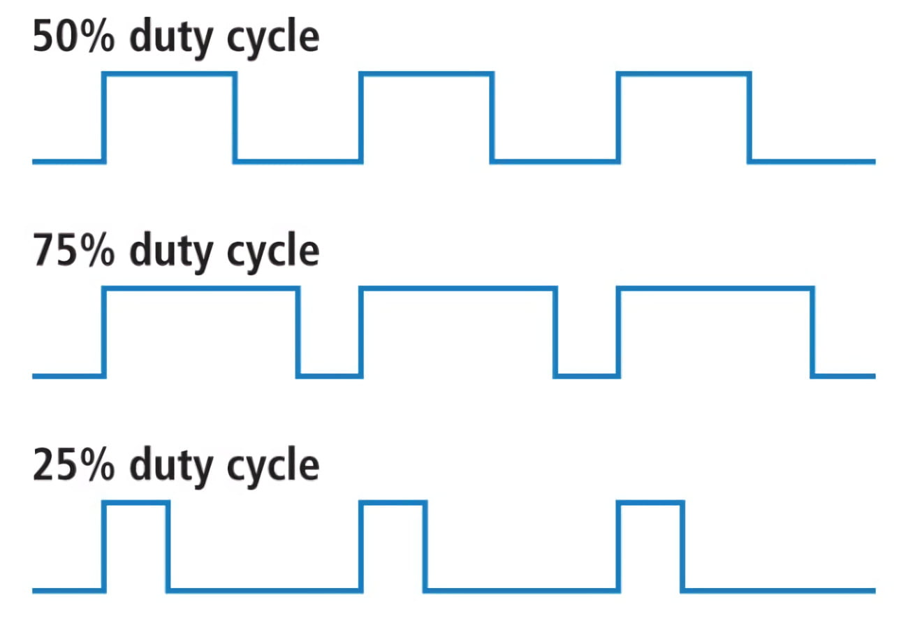
Pulse Width Modulation (PWM) is a technique for generating a continuous HIGH/LOW alternating digital signal and programmatically controlling its pulse width and frequency. Certain loads like (LEDs, Motors, etc) will respond to the average voltage of the signal which gets higher as the PWM signal’s pulse width is increased. This technique is widely used in embedded systems to control LEDs brightness, motor speed, and other applications.
> DeepblueMbedded.com
On the embedded subteam, we use PWM to control the motors for the Robotic arm and Drive system. In the world of PWM, two metrics are most important: duty cycle and frequency. The duty cycle is determined by the percentage of high/low signal, for example a 75% duty cycle means that the signal is HIGH 75% of the time. How long this total time is, is determined by the frequency. The frequency is to determine motor speed.
CubeMX
Make sure you have set up Ethernet according to the following page FIRST: Introduction and initial setup of embedded ethernet
1) Setting Pins
The only pin that is set at the moment (except for defaults) is PA0. It is set to TIM2_CH1, this means it uses Timer 2 Channel 1 for something, in this case it is PWM generation.
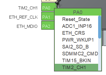
If we want to set more pins to generate PWM signals, we can use a workflow similar to what will be described below. Of course, you will need to choose a separate timer for each pin. Also make sure that the pin is suitable for PWM!
TIM2 > Mode
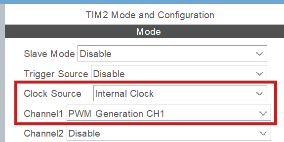
After you have set the pin, you need to enable the timer and channel to do something. We set Clock Source: Internal Clock to enable the timer and Channel1: PWM Generation CH1 to use PWM on pin PA0.
TIM2 > Configuration > NVIC settings
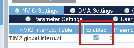
Enable global interrupt.
TIM2 > Configuration > Parameter settings > Counter settings
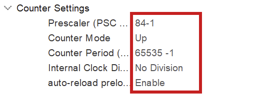
NOTE: -1 for prescaler and counter period because of 0 index counting
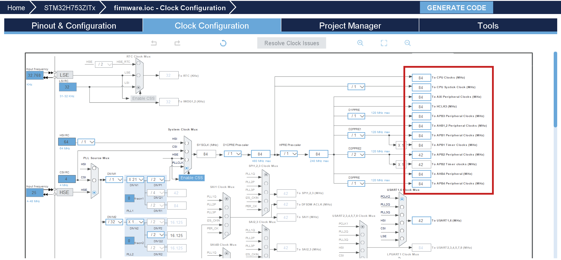
To fully configure the PWM generation, we have to set the above parameters. The prescaler has to do with the clock configuration. You want to set the prescaler equal to the amount of MHz in the clock configuration, because we will divide the clock frequency by the prescaler! Here, we have set the clock speed to 84 MHz (see Clock configuration), so we set the prescaler to 84 (-1) as well. This way we work with 1MHz in calculating the counter period for the wished for PWM frequency (see below).
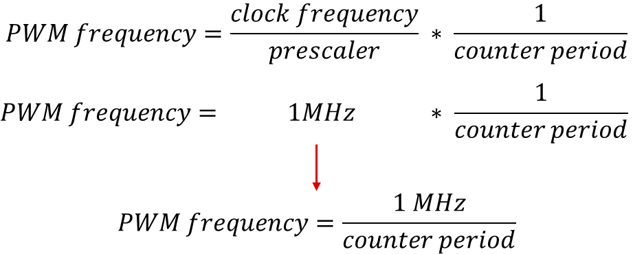
NOTE: the counter period parameter uses the ARR (AutoReload Register). Those terms are used interchangeably in online sources.
As of now, the counter period is at 65535, which is the maximum value for an unsigned 16bit integer. This results in a PWM frequency of 1098Hz. The frequency of PWM should be suitable for the motor you are using. We can change this value later. For more information on PWM see resource 1.
2) Clock configuration
The board can be optimized to run at a higher frequency than is preconfigured. You can set the system clock to work at 84 MHz by setting any of the right-hand clocks in the clock configuration menu to 84. The program then auto calculates the settings for the system, also see resource 2.
Resources
- Deepbluembedded.com: STM32 PWM Output Example Code (PWM Generation Tutorial)
- YouTube: STM32 Beginners Guide Part3: PWM, TIMERS, Frequency and Duty Cycle. LED Dimming with PWM example.
Stepper library
Purpose
CubeMX
1) PWM
NOTE: If you are new to PWM, first take a look at Example PWM generation, it is more in depth
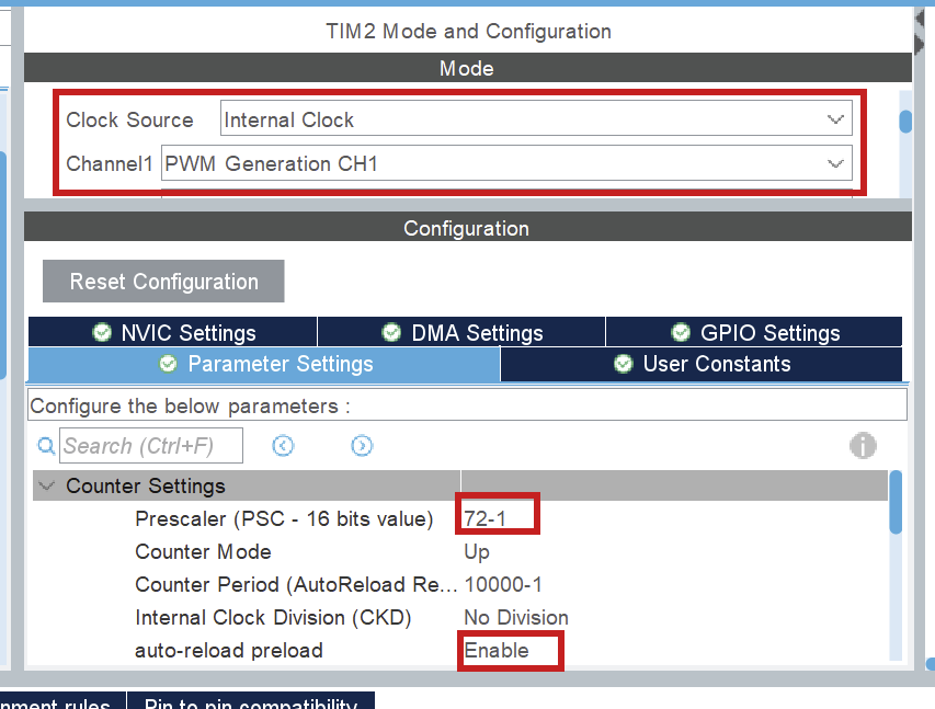
For each stepper, enable pwm on channel 1. This is done by setting Clock Source = Internal Clock and Channel 1 = PWM Generation CH1.
NOTE: Each pwm output for each stepper needs a separate timer. Right now, it is hardcoded that PWM uses Channel 1, so only use Channel 1!
The following parameters are important:
prescaler
The prescaler has to do with the clock configuration. You want to set the prescaler equal to the amount of MHz in the clock configuration, because we will divide the clock frequency by the prescaler! (On the board right now, the clock speeds is set to 72MHz.) This way we work with 1MHz in calculating the frequency and duty cycle.auto-reload preload
I lowkey don't know what this does, just enable it to be safe.
2) DMA
Now, you have to set up the DMA for the same timer/channel. This is in the DMA settings tab.
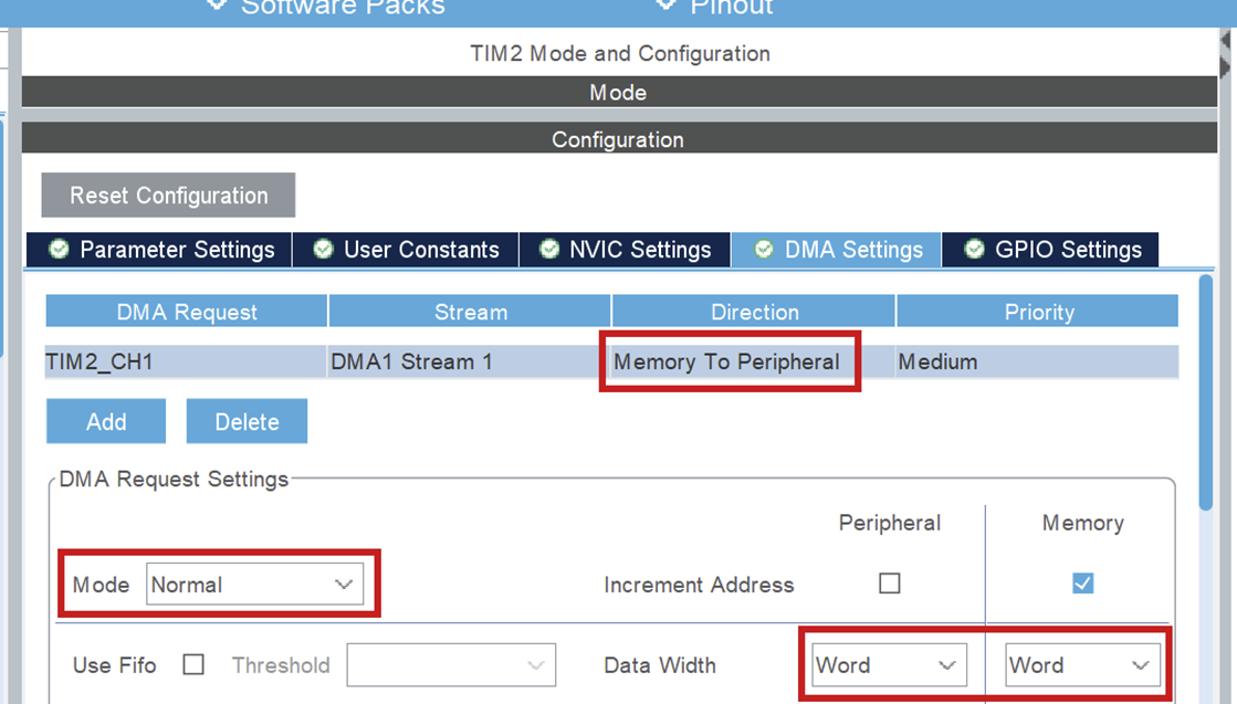
Set the following parameters:
DMA Request = TIMx_CH1
This is the timer and channel which will be using DMA. Make sure this is on channel 1, as stated above!Stream
This can be any of the available streams.Direction = Memory to Peripheral
Important! Because we will be using DMA to transfer PWM signals from the code (memory) to the pin (peripheral) it needs to be set this way.Priority
This can be set to any level, but note that it is advisable to put all steppers to the same priority. I don't know (and am not responsible for) what happens if they are different.Mode = Normal
In normal mode, DMA transfers the buffer from memory ONCE and then remains at the last sent value (remember this, it is important later). See resource 1.Data width = Word
This is the width of the values we will be sending. Since the values we will be sending are used to fill the CCR register, we will set this to word (uint32_t size). Half word would be for 16 bit registers.
3) GPIO pins
Set 2 pins to GPIO_Output by clicking on them in the CubeMX UI. One of these will be used for the direction pin and another for the enable pin.
//TODO: add driver resource
4) Clock Configuration
For PWM it really doesn't matter at what speed you set the clock. The only thing that matters is that the prescalar is set to the same amount. So if your clock speed is 72, set it to 72-1, if your clock speed is 84, set it to 84-1.
Code
1) Public Methods
2) Private Methods
3) Example
Resources
Main
All resources
Control
Overview
General structure
The general structure of how the control system is made, tested, and deployed works like this:
The control system is made using Simulink, using mostly the base functionality to calculate the needed values for different parts of control. Once the general control system is implemented, it is either tested directly in Simulink, mostly using different parts from the Simscape suite to simulate the hardware, or it can be tested by generating the code, and using that code in a separate, more high level simulation program like Gazebo or Webots.
The deployment is mostly managed by the embedded team, as once the code is generated, it can be used in whatever is necessary for the embedded team.
Required software
MATLAB Simulink with the following add-ons:
- Embedded Coder
- Simulink Coder
- Simulink Compiler
- MATLAB Coder
- MATLAB Compiler
Code generation
In general the code is generated from Simulink blocks, where all the control has to do is done inside this one block:
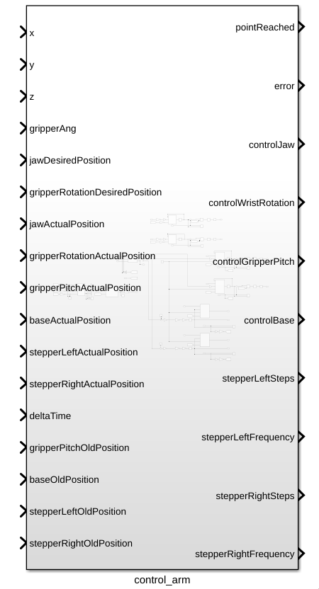
To be able to generate C code for the STM32's you will first need to activate the embedded C coder, which can be done by clicking on the apps tab in the top bar, and then searching for C embedded coder in the apps bar.

After the embedded C coder is active, a new tab called C CODE appears, where you now have to press the quick start button to start the code generation process:

When in the quick start menu, the only critical options for this project are to set the system which gets generated to the main control block of this project, and to set the word size to be the same as the ones from the STM32.
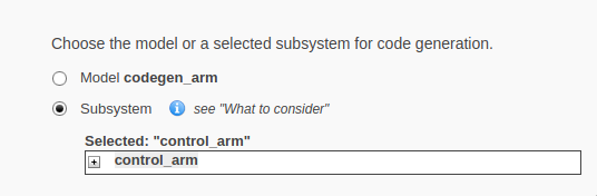
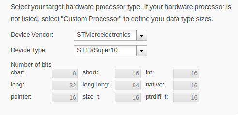
The rest of the settings work best on the default option, but can be changed if deemed necessary.
Automatic control
Overview
In general, the job of the control system is to turn high level instructions from the software system, and turn them into instructions for the hardware. This is done by having a positions in 3d space (x, y z), a final gripper angle (respective to the ground), controls for the rotation, controls for opening and closing the gripper, and a deltaTime as an input, and turning those into control signals for the motors:
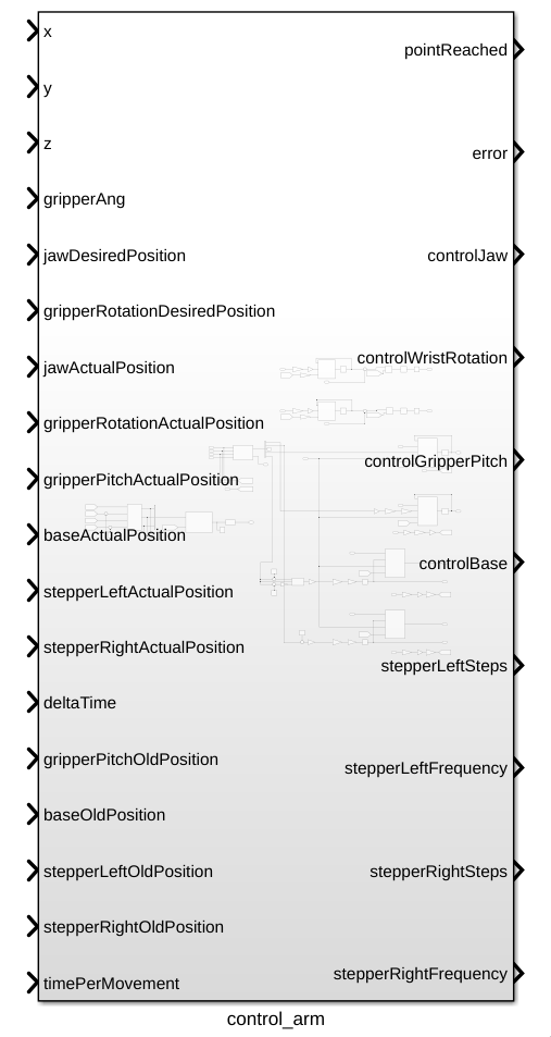
The control system also has feedback from the motors with variables with a name ending with ActualPosition, and the old positions of the motors, representing the position of the motors before the movement starts.
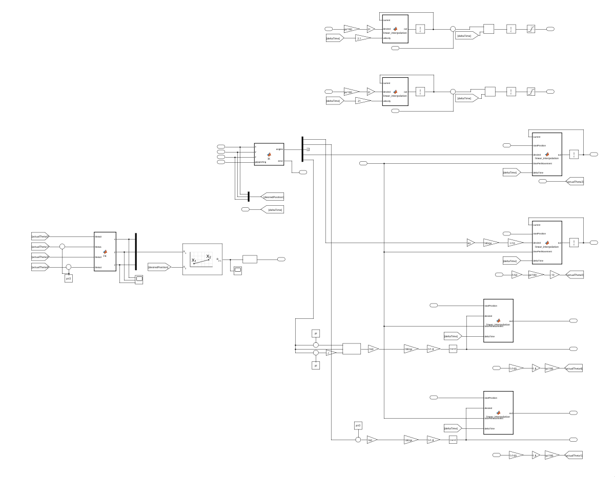
The movement starts whenever the input variables are changed, the old positions must come from an external source, and stay constant throughout the movement.
Inverse kinematics
Starting of the process is the inverse kinematics, which is a matlab function block that calculates the necessary angles that the joints need to make given a final position.
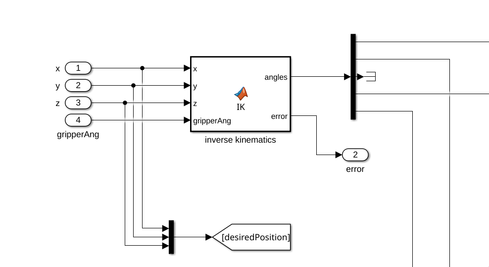
More information about how the inverse kinematics are done can be found in Kinematics.
After that, angles will be sent to the different motor control systems, where they will be processes as a desired position.
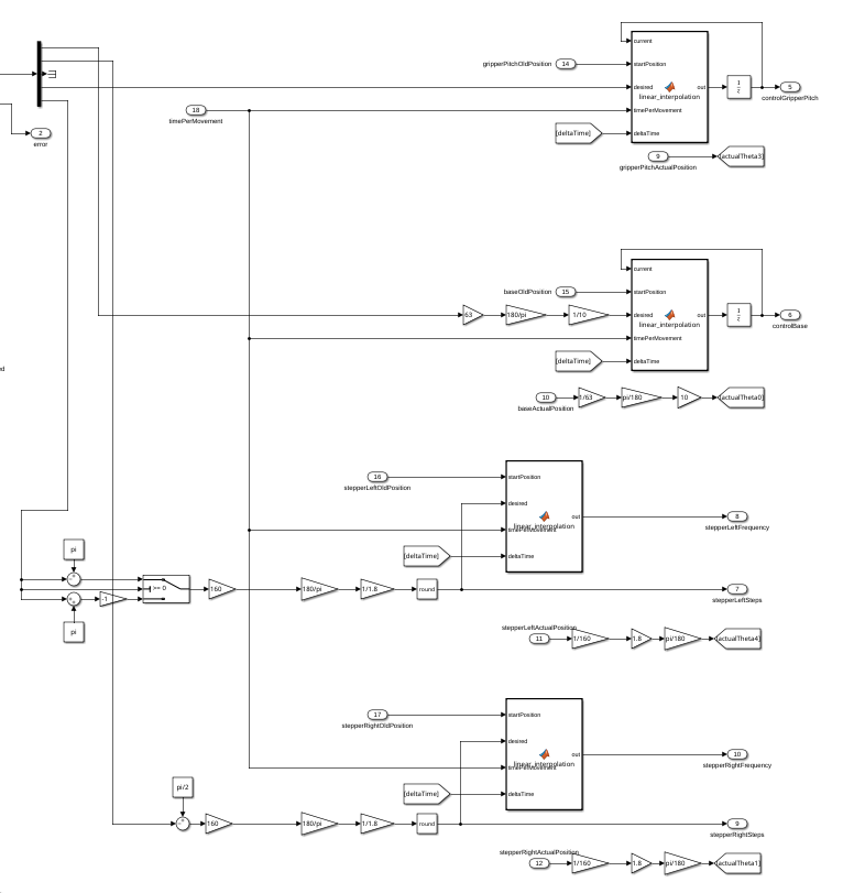
Here you will find a Time per movement constant, that will determine the speed at which a movement will be made. This is necessary to allow the motors to finish a movement at the same time, to minimize positioning issues.
Control signals
DC motors
The controllers used for DC motor control use a Matlab function to linearly interpolate the movement, to allow for a smooth movement. It uses a start position, end position, and current position do determine how fast the motor should move.
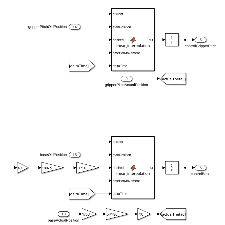
The gain blocks going into the desired inputs are used to take into account the gearboxes attached to these motors (63:1 gear ratio means move 63 times further).
After the linear interpolation, the motor will be controlled using simple PI controllers, using the actual position from the encoders as control input. The actual positions will also be used for forward kinematics later, so they are sent to goto statements.
The linear interpolation works like this:
function out = linear_interpolation(current, startPosition, desired, timePerMovement, deltaTime)

velocity = abs(desired - startPosition) / timePerMovement;

if current < desired
    current = current + (velocity * deltaTime);
end
if current > desired
    current = current - (velocity * deltaTime);
end

out = current;
The motors not used for positioning of the gripper (gripper rotation and jaw control) are also controlled using a linearly interpolated signal, but the velocity of these movements can be varied much more, because they are not dependent on the movement of the rest of the arm.
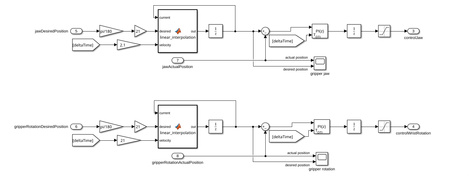
After the linear interpolation, the motors are controlled with PI controllers.
The gain blocks in front of the desired position are scaled to account for an input of degrees, and to account for the gear ratios of the motors. The velocities were arbitrarily picked.
The linear interpolation block works like this:
function out = linear_interpolation(current, desired, velocity)
if current < desired
    current = current + velocity;
end
if current > desired
    current = current - velocity;
end

out = current;
Stepper motors
The stepper motor control works fairly similar, but instead of sending control signals with a PI controller, it just sends the absolute position in terms of steps and the frequency at which the PWM signal should pulse.
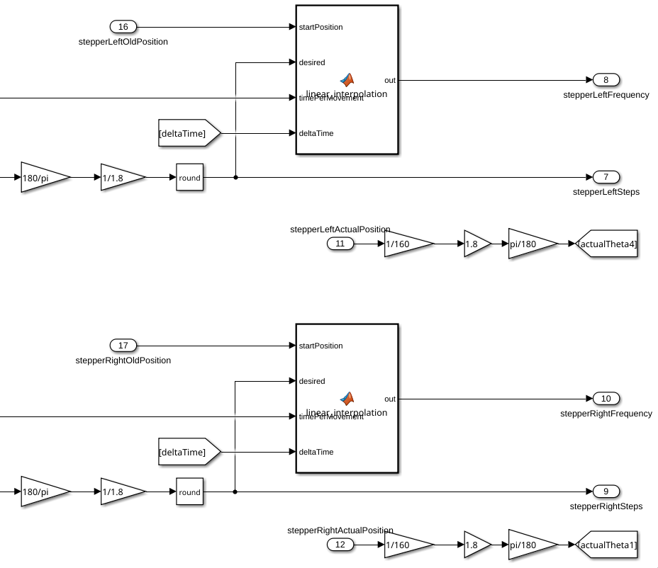
Before getting the desired position though, three gain block are used beforehand, to convert the angle gotten from the inverse kinematics to the position the motor should go to. In this process a, pi/2 gets added to the angle because of how they are calculated.
The gain blocks are here for this reason: 160 is because of the gear ratio between the motor and the actual movement, 180/pi is to convert from radians to degrees, and 1/1.8 is to convert from degrees to steps (these could have been one gain block, but it is more clear why they are here like this).
The frequency calculating function block works like this:
function out = linear_interpolation(startPosition, desired, timePerMovement, deltaTime)

velocity = abs(desired - startPosition) / timePerMovement;

out = velocity;
To confirm the robotic arm has reached the final position it has to, a forward kinematics function is used to get the projected position, which is then compared to the desired position.
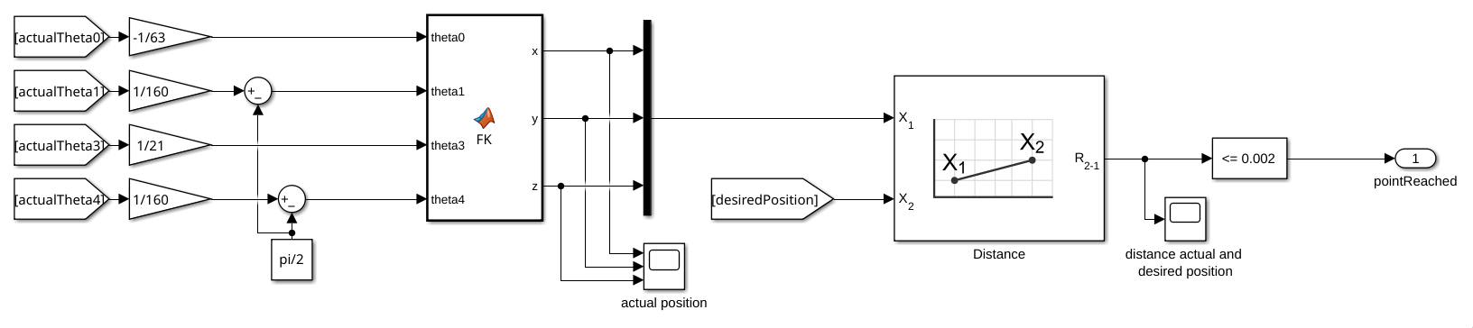
It does forward kinematics on the read values from the encoders, for that reason they have been scaled down to account for the gear ratios (pi/2 is subtracted from theta1 and theta4 because how the encoders are calibrated).
More on how the forward kinematics actually works in Kinematics.
Manual control
Overview
In general, the job of the control system is to turn high level instructions from the software system, and turn them into instructions for the hardware. This is done by having a positions in 3d space (x, y z), a final gripper angle (respective to the ground), controls for the rotation, controls for opening and closing the gripper, and a deltaTime as an input, and turning those into control signals for the motors:
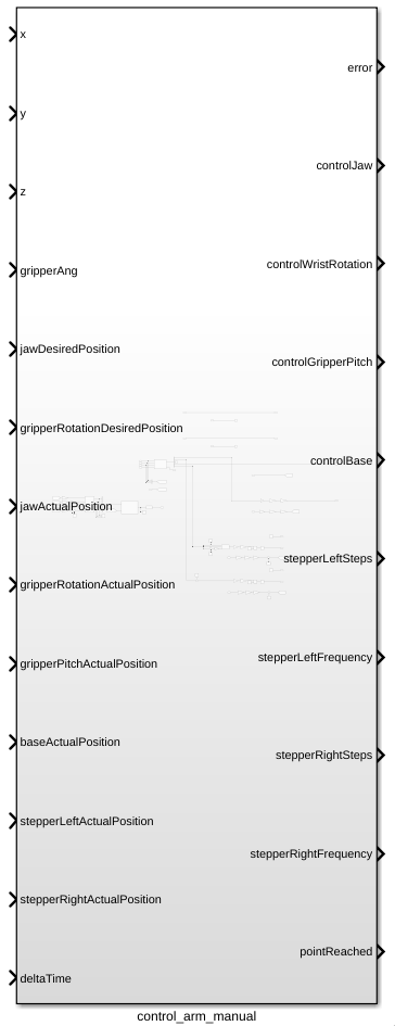
The control system also has feedback from the motors with variables with a name ending with ActualPosition, and the old positions of the motors, representing the position of the motors before the movement starts.
The movement starts whenever the input variables are changed, the old positions must come from an external source, and stay constant throughout the movement.
Inverse kinematics
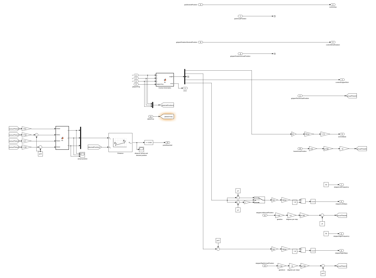
Starting of the process is the inverse kinematics, which is a Matlab function block that calculates the necessary angles that the joints need to make given a final position.
More information about how the inverse kinematics are done can be found in Kinematics.
After that, angles will be sent to the different motor control systems, where they will be processes as a desired position.
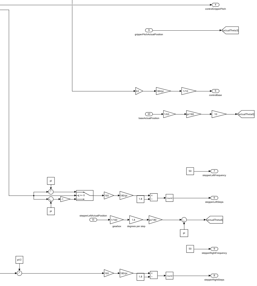
Most of the values are sent straight to the motor drivers, as they are processes by them.
Control signals
DC motors
The DC motors of the robotic arm are all controlled by sending the desired position to them incrementally.
Stepper motors
The stepper motor control works fairly similar, but instead of sending control signals with a PI controller, it just sends the absolute position in terms of steps and the frequency at which the PWM signal should pulse.
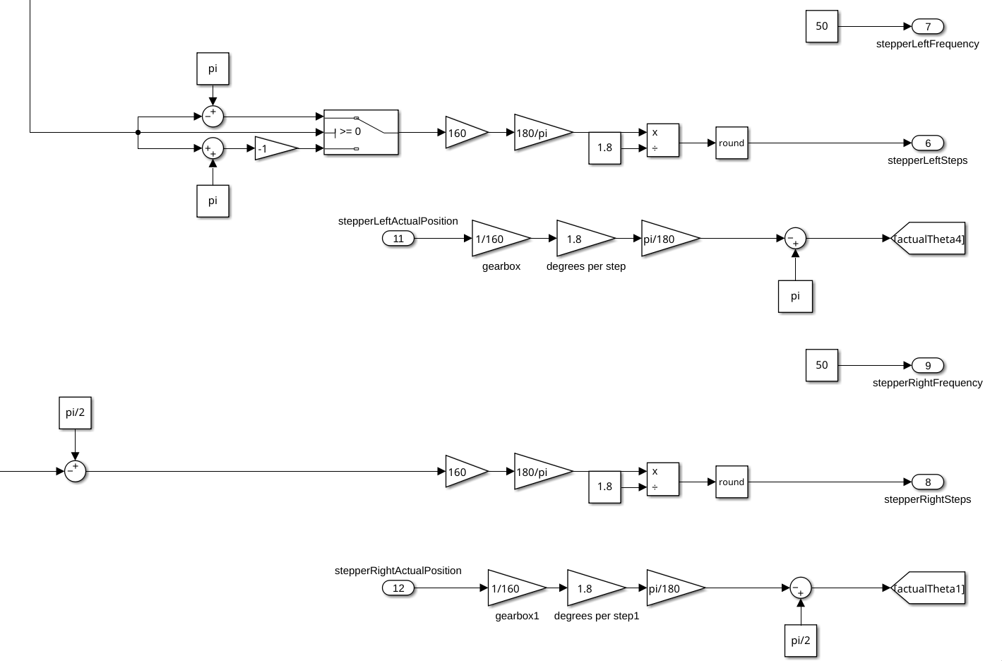
Before getting the desired position though, three gain block are used beforehand, to convert the angle gotten from the inverse kinematics to the position the motor should go to. In this process a, pi/2 gets added to the angle because of how they are calculated.
The gain blocks are here for this reason: 160 is because of the gear ratio between the motor and the actual movement, 180/pi is to convert from radians to degrees, and 1/1.8 is to convert from degrees to steps (these could have been one gain block, but it is more clear why they are here like this).
To confirm the robotic arm has reached the final position it has to, a forward kinematics function is used to get the projected position, which is then compared to the desired position.
It does forward kinematics on the read values from the encoders, for that reason they have been scaled down to account for the gear ratios (pi/2 is subtracted from theta1 and theta4 because how the encoders are calibrated).
More on how the forward kinematics actually works in Kinematics.
Kinematics
Defining terms
To do kinematics on the robotic arm, it first needs to be modelled in a way to do calculations on the different joint angles and positions. This is done by using 4x4 matrix notation to represent the different joints.
The different points and angles are defined like this:
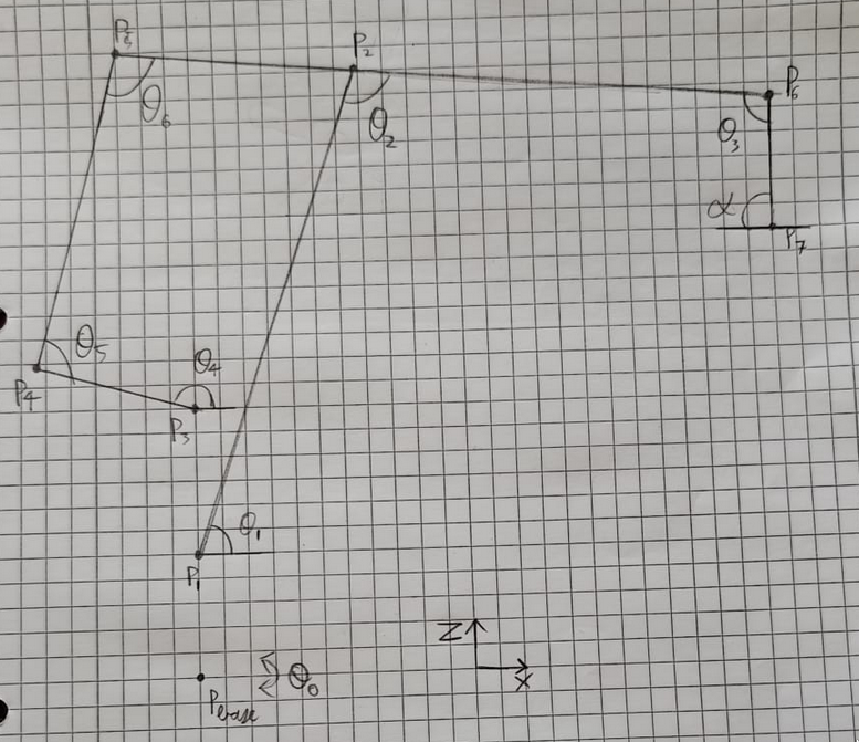
In the all the following code blocks, there will be different types of variables used.
Variables that start with a P represent points,
variables that start with a T represent transform that can be performed on points,
and variables that start with an L are scalar length values.
Note: all angles are measured in radians, and all lengths are measured in meters.
Forward kinematics
The input arguments of the function are the actuated angles of the arm, since these are the only ones measurable by the encoders.
The function returns the projected end position of the end effector.
function [x, y, z] = forward_kinematics(theta0, theta1, theta3, theta4)
    %defining dimentions
    LbaseToP1 = 0.065;
    LbaseToP3 = 0.149;

    LP1toP2 = 0.350;
    LP5toP6 = 0.620;
    LP5toP2 = 0.120;
    LP6toP7 = 0.300;

    LP3toP4 = 0.120;
    LP4toP5 = 0.280;
The first thing that happens in the forward kinematics is the definition of the dimensions of the different joints, these values are gotten from measuring the physical arm.
The point representing the base rotation (Pbase) is rotated theta0 radians.
    %rotation z
    TP0toPbase = [cos(theta0) -sin(theta0) 0 0;
                  sin(theta0)  cos(theta0) 0 0;
                  0            0           1 0;
                  0            0           0 1];
From there, all the known transforms to the different points are defined, the transforms are defined with the main idea being, rotation happens along the Z-axis, and translation happens along the X-axis. This is done by first translating shoulder actuated points (P1 and P3) and then rotating them along the x axis.
    %translation z then rotation x
    TPbasetoP1 = [1 0 0  0;
                  0 0 -1 0;
                  0 1 0  LbaseToP1;
                  0 0 0  1];

    %rotation z
    TPbasetoP1 = TPbasetoP1 * [cos(theta1) -sin(theta1) 0 0;
                               sin(theta1)  cos(theta1) 0 0;
                               0            0           1 0;
                               0            0           0 1];
%translation z then rotation x
TPbasetoP3 = [1 0 0 0;
0 0 -1 0;
0 1 0 LbaseToP3;
0 0 0 1];
%rotation z
TPbasetoP3 = TPbasetoP3 * [cos(theta4) -sin(theta4) 0 0;
sin(theta4) cos(theta4) 0 0;
0 0 1 0;
0 0 0 1];The reason that they are rotated twice is because it is easier to keep track of the relative positions and angles involved.
After that, the other currently inferrable transforms are defined.
    %translation x
    TP1toP2 = [1 0 0 LP1toP2;
               0 1 0 0;
               0 0 1 0;
               0 0 0 1];

    %translation x then rotation z
    TP5toP6 = [cos(theta3) -sin(theta3) 0 LP5toP6;
               sin(theta3)  cos(theta3) 0 0;
               0            0           1 0;
               0            0           0 1];

    %translation x
    TP6toP7 = [1 0 0 LP6toP7;
               0 1 0 0;
               0 0 1 0;
               0 0 0 1];

    %translation x
    TP3toP4 = [1 0 0 LP3toP4;
               0 1 0 0;
               0 0 1 0;
               0 0 0 1];
Some of these transforms don't have rotations, this is because we either don't know the angle rotation yet, or it is an end point, that does not have to be moved and by extension rotated further.
Due to the construction of the arm, some calculations have to be done to find the rest of the unknown angles.
This is done by first defining an initial position, and then some theoretical "planar" positions of the points P2 and P4.
    %initial position
    P0 = [1 0 0 0;
          0 1 0 0;
          0 0 1 0;
          0 0 0 1];

    %getting position for paralellagram angles
    P2planar = P0 * TPbasetoP1 * TP1toP2;
    P4planar = P0 * TPbasetoP3 * TP3toP4;
The reason they are planar is because they were produces without any base rotation, so they all lay on the y=0 plane.
After that, a small inverse kinematics equation is performed to find the angles theta5 and theta6, which is done using a standard formula.
    L_1 = LP4toP5; L_2 = LP5toP2;
    XE = P4planar(1, 4) - P2planar(1, 4);
    YE = P4planar(3, 4) - P2planar(3, 4);
    theta5 = 2*atan((2*L_1*YE + sqrt(- L_1^4 + 2*L_1^2*L_2^2 + 2*L_1^2*XE^2 + 2*L_1^2*YE^2 - L_2^4 + 2*L_2^2*XE^2 + 2*L_2^2*YE^2 - XE^4 - 2*XE^2*YE^2 - YE^4))/(L_1^2 + 2*L_1*XE - L_2^2 + XE^2 + YE^2));
    theta6 = -2*atan(sqrt((- L_1^2 + 2*L_1*L_2 - L_2^2 + XE^2 + YE^2)*(L_1^2 + 2*L_1*L_2 + L_2^2 - XE^2 - YE^2))/(- L_1^2 + 2*L_1*L_2 - L_2^2 + XE^2 + YE^2));
    %adding pi-theta4 to make the actual rotation angle
    theta5 = theta5+(pi-theta4);
Now that we know all the angles, the rest of the transforms can be defined.
    %translation x then rotation z
    TP3toP4 = [cos(theta5) -sin(theta5) 0 LP3toP4;
               sin(theta5)  cos(theta5) 0 0;
               0            0           1 0;
               0            0           0 1];

    %translation x then rotation z
    TP4toP5 = [cos(theta6) -sin(theta6) 0 LP4toP5;
               sin(theta6)  cos(theta6) 0 0;
               0            0           1 0;
               0            0           0 1];
And now we have all the transforms, we can calculate all the points.
    %calculating all needed points
    Pbase = TP0toPbase;
    P3 = Pbase * TPbasetoP3;
    P4 = P3 * TP3toP4;
    P5 = P4 * TP4toP5;
    P6 = P5 * TP5toP6;
    P7 = P6 * TP6toP7;
Finally, the final position of the end effector can be read from the final point.
    %extracting position
    x = P7(1,4);
    y = P7(2,4);
    z = P7(3,4);
end
Inverse kinematics
The inverse kinematics uses the same representation of points and angles to represent the linkages of the arm.
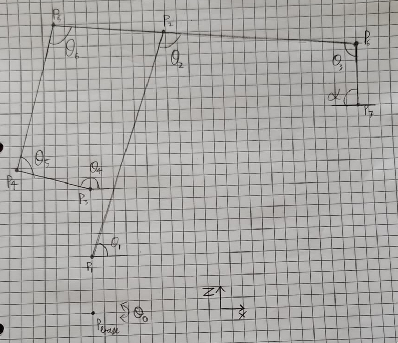
The inputs for this function are the position of the end effector (x, y, z) and a final gripper angle alpha, which is in reference to the ground.
The outputs are the angles of the actuated points as shown above.
The first thing the function does checking a simple error case, as this will not be caught anywhere else otherwise.
function [theta0, theta1, theta3, theta4, error] = inverse_kinematics(x, y, z, alpha)
    defaultAngles = [0; pi/2; 0; -pi/2; pi];
    error = 0;

    if x == 0 && y == 0
        theta0 = defaultAngles(1);
        theta1 = defaultAngles(2);
        %theta2 = defaultAngles(3);
        theta3 = defaultAngles(4);
        theta4 = defaultAngles(5);
        error = 1;
        return;
    end
After that the same dimensions as the forward kinematics are defined.
    %all the lengths are in meters
    LbaseToP1 = 0.065;
    LbaseToP3 = 0.149;

    LP1toP2 = 0.350;
    LP2toP6 = 0.500;
    %LP5toP6 = 0.620;
    LP5toP2 = 0.120;
    LP6toP7 = 0.300;

    LP3toP4 = 0.120;
    LP4toP5 = 0.280;
Since the arm is planar by nature, the angle of the base rotation (theta0) can easily be calculated. A variable called angToBase is also defined, it represents the angle of the end effector to the base of the arm.
    if x < 0
        theta0 = atan(y/x) + pi;
    else
        theta0 = atan(y/x);
    end
    angToBase = theta0 - pi;
After that, P7 and P6 are defined using the input arguments. The rotation x on P7 is to align rotations with the z-axis and translations with the x-axis. (The i at the end is for inverse.)
  %setting end position, rotated towards the base
    P7i = [cos(angToBase) -sin(angToBase) 0 x;
           sin(angToBase)  cos(angToBase) 0 y;
           0               0              1 z;
           0               0              0 1];

    %rotation x
    P7i = P7i * [1 0  0 0;
                 0 0 -1 0;
                 0 1  0 0;
                 0 0  0 1];

    %rotation z
    TP7toP6i = [cos(alpha) -sin(alpha) 0 0;
                sin(alpha)  cos(alpha) 0 0;
                0           0          1 0;
                0           0          0 1];

    %translation x
    TP7toP6i = TP7toP6i * [1 0 0 LP6toP7;
                           0 1 0  0;
                           0 0 1  0;
                           0 0 0  1];

    P6i = P7i * TP7toP6i;
P1 is also defined.
    %translation z
    P1i = [1 0 0 0;
           0 1 0 0;
           0 0 1 LbaseToP1;
           0 0 0 1];
Now that P1, P6, and P7 are defined, they will be used to calculate theta1, theta2, and theta3.
This is done by first checking if this movement would be possible kinematically, and then actually calculating the angles. This is done with the same standard formula shown in the forward kinematics.
    %calculating theta1, theta2 and theta3
    L_1i = LP1toP2; L_2i = LP2toP6;
    dx = P6i(1,4) - P1i(1,4);
    dy = P6i(2,4) - P1i(2,4);
    XEi = sqrt(dx*dx + dy*dy);
    YEi = P6i(3,4) - P1i(3,4);

    if (- L_1i^4 + 2*L_1i^2*L_2i^2 + 2*L_1i^2*XEi^2 + 2*L_1i^2*YEi^2 - L_2i^4 + 2*L_2i^2*XEi^2 + 2*L_2i^2*YEi^2 - XEi^4 - 2*XEi^2*YEi^2 - YEi^4) < 0
        error = 1;
        theta0 = defaultAngles(1);
        theta1 = defaultAngles(2);
        %theta2 = defaultAngles(3);
        theta3 = defaultAngles(4);
        theta4 = defaultAngles(5);
        return;
    end

    theta1 = 2*atan((2*L_1i*YEi + sqrt(- L_1i^4 + 2*L_1i^2*L_2i^2 + 2*L_1i^2*XEi^2 + 2*L_1i^2*YEi^2 - L_2i^4 + 2*L_2i^2*XEi^2 + 2*L_2i^2*YEi^2 - XEi^4 - 2*XEi^2*YEi^2 - YEi^4))/(L_1i^2 + 2*L_1i*XEi - L_2i^2 + XEi^2 + YEi^2));
    theta2 = -2*atan(sqrt((- L_1i^2 + 2*L_1i*L_2i - L_2i^2 + XEi^2 + YEi^2)*(L_1i^2 + 2*L_1i*L_2i + L_2i^2 - XEi^2 - YEi^2))/(- L_1i^2 + 2*L_1i*L_2i - L_2i^2 + XEi^2 + YEi^2));

    theta3 = 2*pi - alpha -theta1 -theta2;
These angles are then used to define transforms to other necessary points. An initial point is also defined.
    %translation z then rotation x
    TPbasetoP1 = [1 0 0  0;
                  0 0 -1 0;
                  0 1 0  LbaseToP1;
                  0 0 0  1];

    %rotation z
    TPbasetoP1 = TPbasetoP1 * [cos(theta1) -sin(theta1) 0 0;
                               sin(theta1)  cos(theta1) 0 0;
                               0            0           1 0;
                               0            0           0 1];

    %translation x then rotation z
    TP1toP2 = [cos(theta2) -sin(theta2) 0 LP1toP2;
               sin(theta2)  cos(theta2) 0 0;
               0            0           1 0;
               0            0           0 1];

    %translation z then rotation x
    TPbasetoP3 = [1 0 0  0;
                  0 0 -1 0;
                  0 1 0  LbaseToP3;
                  0 0 0  1];

    %translation x
    TP2toP5 = [1 0 0 -LP5toP2;
               0 1 0 0;
               0 0 1 0;
               0 0 0 1];

    %initial position
    P0 = [1 0 0 0;
          0 1 0 0;
          0 0 1 0;
          0 0 0 1];
These new transforms are now used to interpolate planar versions of P3 and P5.
    %getting position for paralellagram angles
    P3planar = P0 * TPbasetoP3;
    P5planar = P0 * TPbasetoP1 * TP1toP2 * TP2toP5;
These points are used to calculate the final needed angles, using the same formula as before.
    %getting parallelageram angles
    L_1 = LP3toP4; L_2 = LP4toP5;
    XE = P5planar(1, 4) - P3planar(1, 4);
    YE = P5planar(3, 4) - P3planar(3, 4);

    if (- L_1^4 + 2*L_1^2*L_2^2 + 2*L_1^2*XE^2 + 2*L_1^2*YE^2 - L_2^4 + 2*L_2^2*XE^2 + 2*L_2^2*YE^2 - XE^4 - 2*XE^2*YE^2 - YE^4) < 0
        error = 1;
        theta0 = defaultAngles(1);
        theta1 = defaultAngles(2);
        %theta2 = defaultAngles(3);
        theta3 = defaultAngles(4);
        theta4 = defaultAngles(5);
        return;
    end

    theta4 = 2*atan((2*L_1*YE + sqrt(- L_1^4 + 2*L_1^2*L_2^2 + 2*L_1^2*XE^2 + 2*L_1^2*YE^2 - L_2^4 + 2*L_2^2*XE^2 + 2*L_2^2*YE^2 - XE^4 - 2*XE^2*YE^2 - YE^4))/(L_1^2 + 2*L_1*XE - L_2^2 + XE^2 + YE^2));
Note: the angles resulting from the function are equal to the angles defined on the diagram above, which are not equal to the positions the motors have to move to.
Simulation
Simulink
Overview
The main simulation used for testing the control system of the robotic arm is made with Simulink, using the different parts of the Simscape suite to simulate the robotic arm.
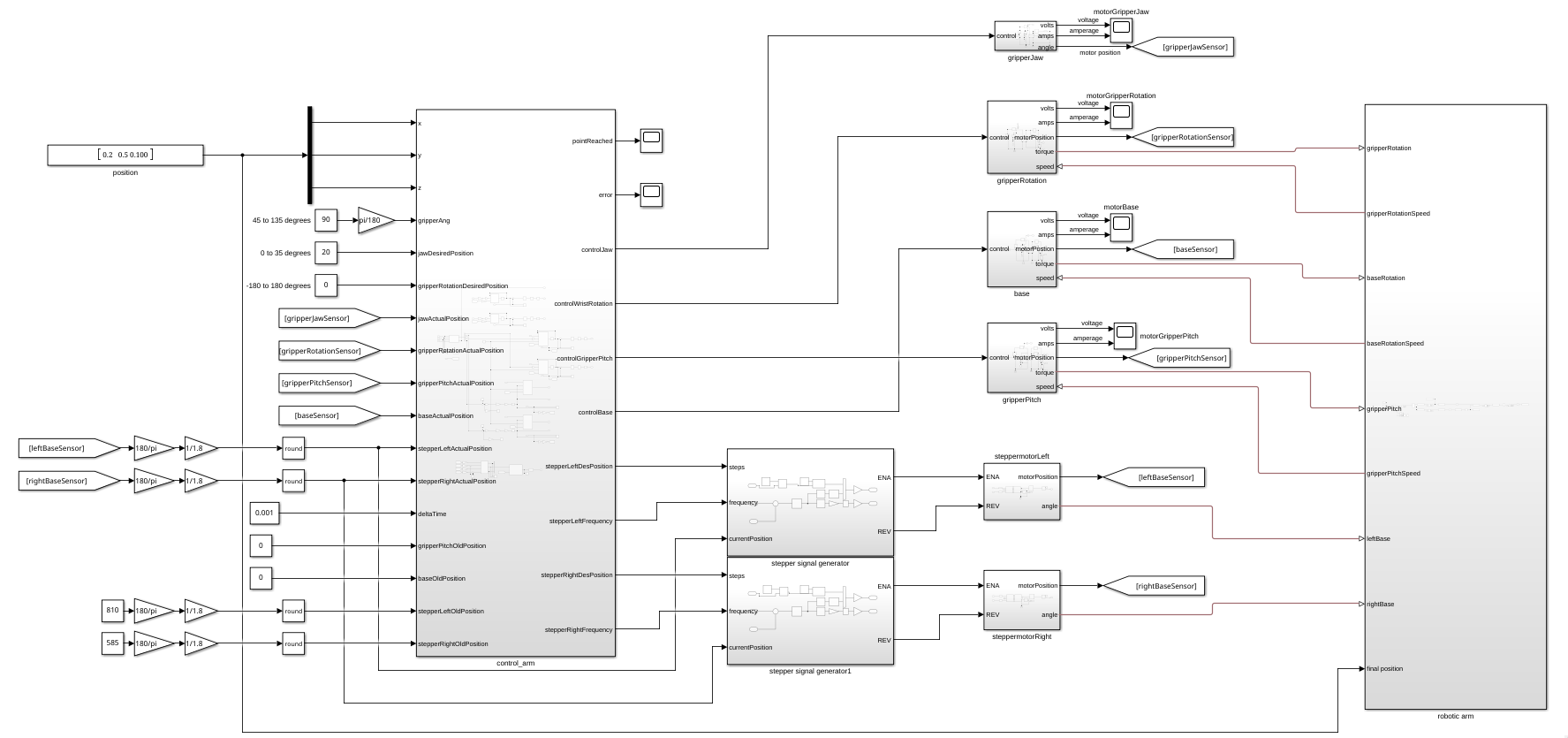
The simulation works by using a main control block that sends instructions to different simulated motors, which are then connected to a 3d model of the robotic arm.
Motors
There are two main types of motors used for simulation, DC motors and stepper motors. All of these parts are simulated using the Simscape suite.
DC motors
The parts controlled by DC motors are the base rotation, gripper pitch, gripper rotation, and gripper jaw (opening and closing).
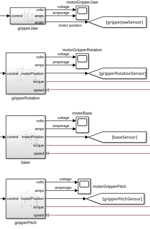
The DC motors are controlled with a control signal that ranges from 0V-5V, which is then converted to a 0V-24V signal that the motor can use. The voltage and amperage going to the motor are measured and sent to outputs to get estimations of how much power the motors will use.
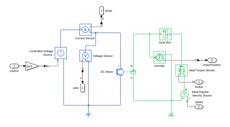
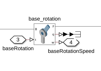
The resulting rotational force is then sent to a gearbox, after which the torque sensor and angular velocity source are used to connect the motor to the model of the arm. The toque sensor is connected to the torque inputs of the joints, and the velocity source is connected to the speed output of the joints.
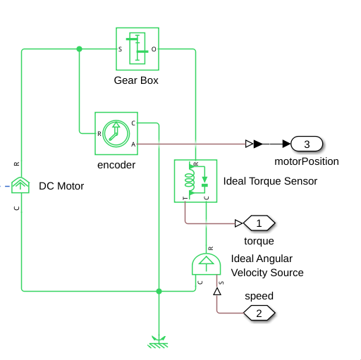
The position of the motor is measured before the gearbox, as this is where the encoder would be on the actual motors.
Since the jaw motors is not currently simulated to move the model of the arm, it has its own simple implementation that takes into account the resistance of the springs that are on the jaws of the gripper.
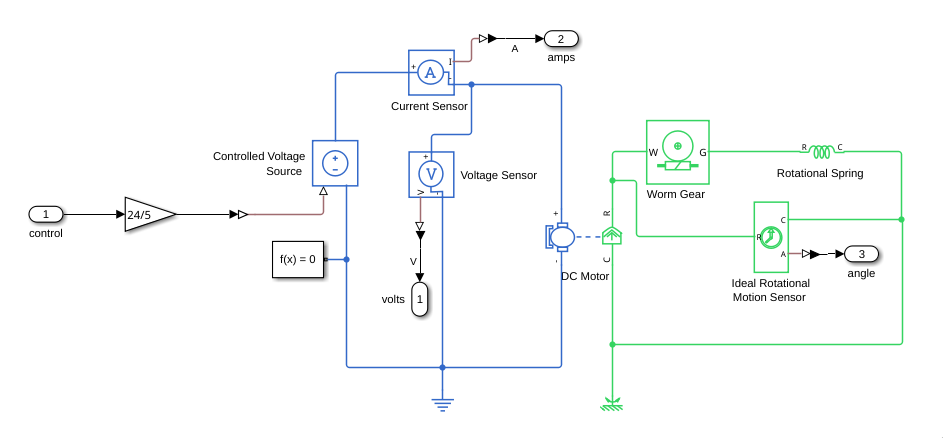
It uses a worm gear and a spring to simulate how the jaws would move without anything in them.
Stepper motors
The two motors in the shoulder joint, actuating the parallelogram construction are stepper motors. These are controlled in two stages, first determining the desired position in terms of steps and the frequency at which the steps should happen, and then generating the steps to make the stepper motors move.
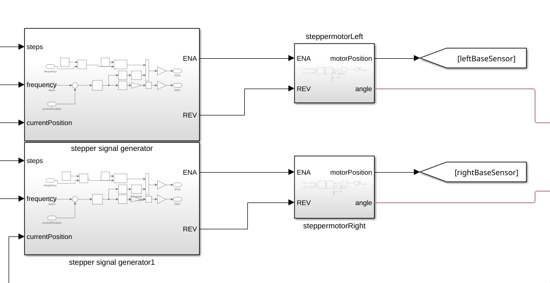
The role of the stepper signal generators is to generate a PWM signal as the STM32's would do given the absolute position and frequency of the steps.
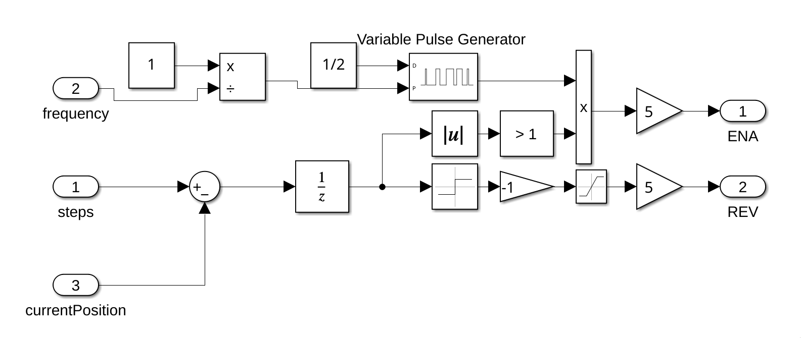
Simply what it does is send pulses at the specified frequency whenever the error between the desired step position is different from the real one.
Note: this way of generating pulses is only for this specific simulation, and would be a bad implementation for anything else.
The stepper motors work by connecting the ENA and REV connections from the previous block to the ENA and REV from a stepper motor driver, which makes the stepper motor move.
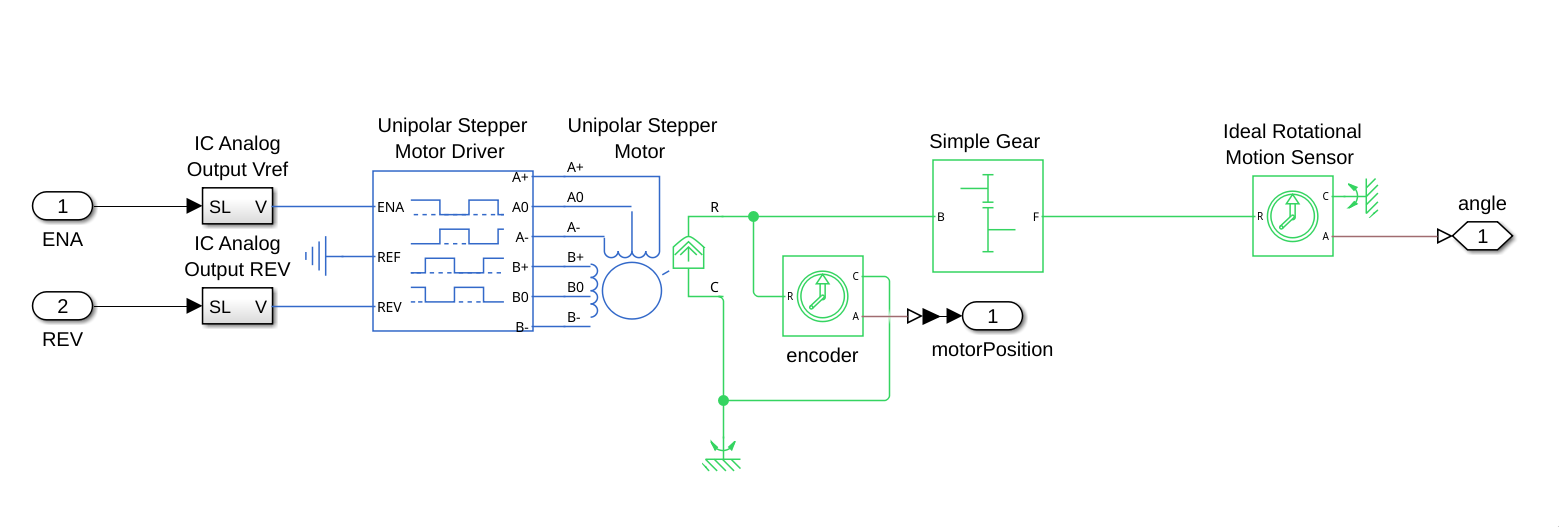
The rotational movement from the stepper motor is read both before and after the gearbox, before to get the encoder values from the motor, and after to use as output to the robotic arm model.
3d model
To show a 3d simulation of the robotic arm, a simplified version of the arm is used. Most of the part models are ported from SolidWorks, using STEP files to render the models. Apart from the gripper, which uses an altered version of the gripper model, and uses two obj files, one for the base and one for the claw, to allow for rotation of the gripper in the simulation.
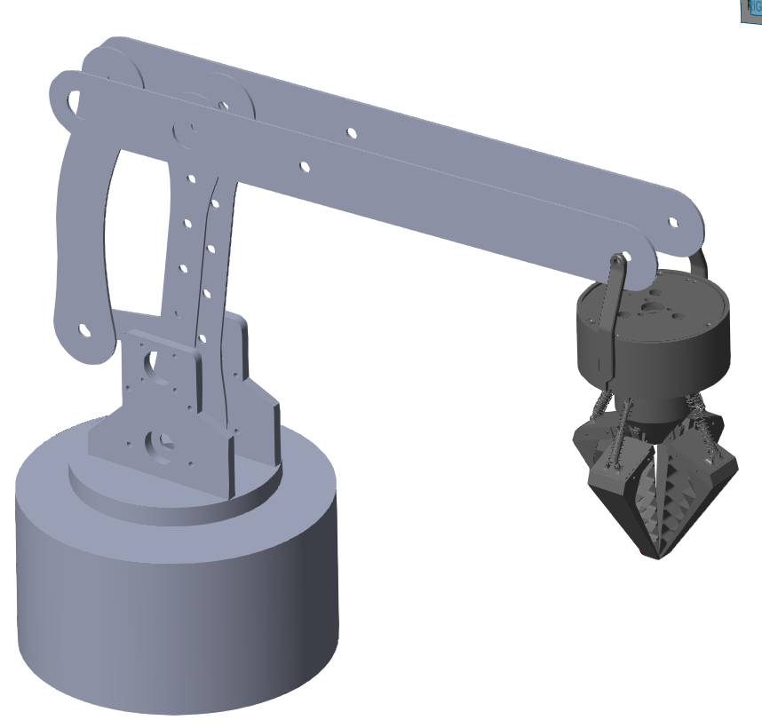
This model is connected to the simulated motors by connecting the physical torque signals the motors produce, and connecting the output speed from the joints back to the motors. This allows the control system to send instructions to the motors, and let the motors then manipulate the arm.
In Simulink, the simulation of the robotic arm by connecting different Simscape parts together with different types of joints.

Each of the white blocks are parts, and the joints, due to the nature of the arm, are all revolute joints.
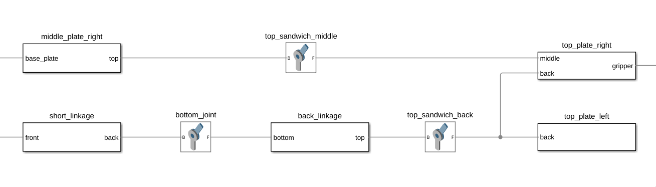
The different parts work by having a rigid transform from one attachment point to the other, as well as a reference point and a model file, to show how the arm would actually look like.
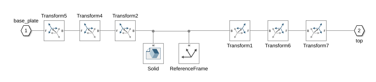
The actuated joints are connected to connection points that connect to the motors from outside of the model block.
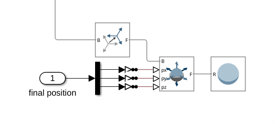
The model also includes a red ball that is moved to the desired position of the end effector, which in this case is the tip of the gripper.
Webots
Instructions for using the webots simulation can be found on the github page of the simulation.
Mechanics
Base
Parallel Linkage
1. Requirements
The structure of the robotic arm is the connection point between the rover and the end-manipulator. Hence, it is crucial to aim for a large reach and a lightweight dynamic structure that can support the loaded gripper and allow for precise motion. During the academic year 2025-2026, the aim was to develop Before starting the design phase, a list of requirements was set:
(a) The robotic arm shall reach a distance of around 1 meter when fully extended in any direction.
(b) The robotic arm shall aim for an overall lightweight design (less than 10kg)
(c) The robotic arm shall be easy to mount on the rover (5-10 minutes mounting time)
(d) The robotic arm shall be easy to disassemble (<30 minutes)
(e) The robotic arm shall be easy to assemble (<30 minutes)
(f) The mounting of all actuators shall consider cable management.
(g) Off-the-shelf components are prioritised during design and assembly
(h) The manufacturing of all parts shall be possible within the university infrastructures
2. Concept & Motivation
A parallel linkage was chosen as the structure of the robotic arm for weight reduction purposes. During early design phases, it was observed that the shoulder motor (see Figure 1) would require significantly higher torque requirements to handle the rest of the arm. These high torque requirements are induced by the considerable length of the robotic arm (aiming for a reach of around 1 m) but also because of the weight created by the elbow motor that results in a significant increase in inertia.
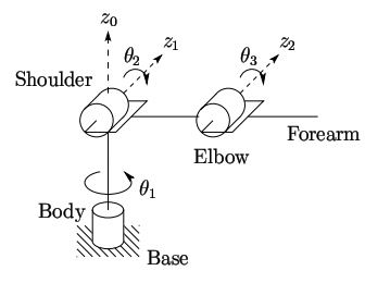
Figure 1: Kinematic diagram of traditional robotic arms and joint names [1].
To address these challenges, we opted to utilise a parallel linkage for the robotic arm's structure (see Figure 2). This structure groups the 2DOFs (θ2 and θ3) at the base of the linkage, minimising the inertia of the entire robotic arm. The disadvantages of this structure include a reduced reach, as it is physically challenging to extend the arm fully, but also a less instinctive arm design that might result in control challenges. After evaluating all factors influencing the design (motor selection, design components and manufacturing), it was decided that the parallel linkage remains an interesting trade-off for the whole system and hence was selected as the final concept.
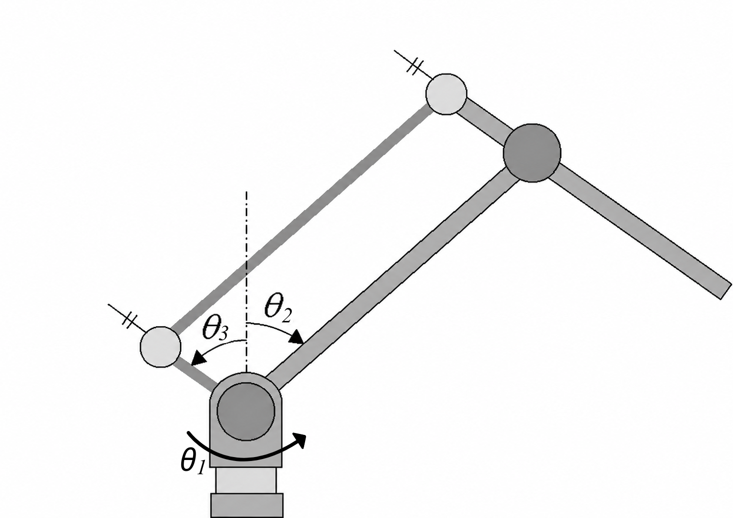 Figure 2: Kinematic diagram of parallel linkage [2].
3. Design & Materials
Figure 3 shows the final execution of the parallel linkage concept presented in the last section. A 3D-printed circular base is used as a connection point with the Base assembly. Four 3D-printed vertical plates are used to mount the two motors and gearboxes that actuate the two shoulder actuations (θ2 and θ3). The wrist actuation of the end-manipulator (moving the gripper up and down, see the Gripper page) uses a DC motor located in the middle of the forearm to reduce inertia and avoid mounting the gripper directly on the motor. A 1:1 belt drive transfers the torque from the DC motor to the gripper.
All plates used in the parallel linkage were laser-cut from 3 mm-thick aluminium sheets ordered from MCB Direct. All shafts that were not included in a motor or a gearbox were turned at CUBE, from raw material ordered from RS. Five deep-groove ball bearings were used to support all moving shafts within the parallel linkage (16101). All pulleys are 3D-printed due to manufacturing challenges to fit the gearbox and motor shafts. The belts were ordered from RS. The aluminium sheets are mounted and held together by standoffs from RS. This structure is called a 'sandwich'. The top sandwich (or forearm) uses a combination of two M4 standoffs (50 mm and 60 mm) to reach a size of 110mm. The bottom sandwich uses M4x40 mm standoffs.
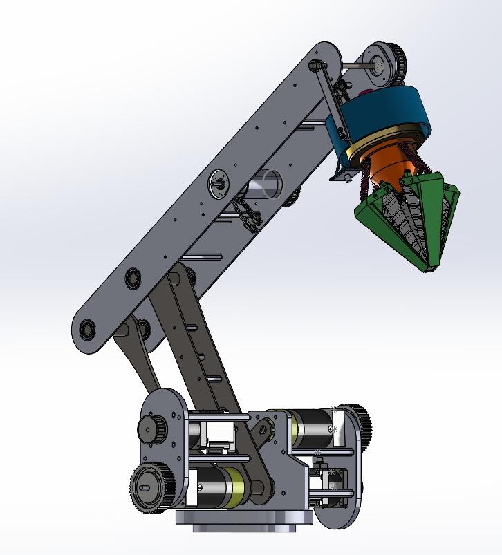
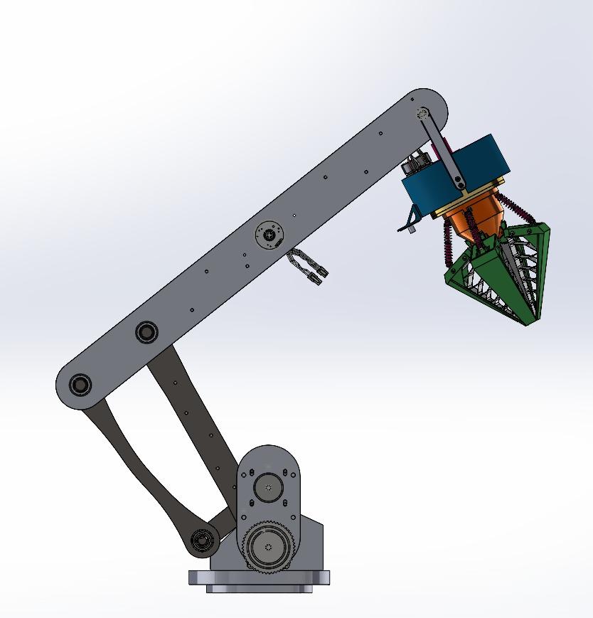
spacespacespacespacespa(a)spacespacespacespacespacespacespacespacespacespace (b)
Figure 3: Full assembly of the parallel linkage, where (a) shows the connections with the shoulder motor and gearboxes, the integration of the wrist motor, and the connection to the gripper, and (b) shows the side view of the assembly, where the final design of the parallel linkage is clearly visible.
The stepper motors (ST5918M3008-B) and gearboxes (GPLE60-3S-80) actuating the shoulder DOFs are from Nanotec. Additionally, the stepper motors were ordered with an additional encoder (NTO3-05-C06 (6.35 mm)) and brake (BRAKE-BCD56-1,5-8). The wrist motor (AK45-10) was bought from CubeMars.
References:
[1] Gupta, Ayush & Chourika, Sameer & Agrawal, Sankalp & Deshmukh, Ankur & Bhargava, Prasham. (2018). A Geometric Approach to Inverse Kinematics of a 3 DOF Robotic Arm.
[2] Ahn, Kuk‐Hyun et al. “Reduction in gravitational torques of an industrial robot equipped with 2 DOF passive counterbalance mechanisms.” 2016 IEEE/RSJ International Conference on Intelligent Robots and Systems (IROS) (2016): 4344-4349.
Gripper
The first version of the gripper was designed and prototyped for a minor assignment with PD&D (Product Design & Development). The full report includes the detailed Literature review, Conceptualisation, Concept Evaluation, Design and Prototyping Phase, as well as motor choices, transmission ratios, and material selections. The report can be found in the Roboteam Twente 2025-2026 folder at the following location:
The report can also be found by clicking on the following link:
1. Summary & Content of report
A) Literature Review
Various existing manipulator technologies, including parallel jaw grippers, underactuated dexterous hands, and soft grippers such as those utilizing the Fin-Ray Effect (FRE) were researched and analysed. The review also evaluates actuation systems, comparing traditional gearboxes with high-efficiency cycloidal and harmonic drives, and contrasting electric motors with pneumatic alternatives.
B) Conceptualization
Six initial concepts were proposed and evaluated using a weighted rating system. The evaluation identified the strengths of FRE jaws (Concept 6) and the planetary gearbox rotation mechanism (Concept 4). These were combined into a final hybrid design (Concept 7), which achieved the highest overall score for its balance of compliance, torque, and weight.
C) Design and Justification
This section details the mechanical architecture of the final gripper, featuring branched FRE jaws for maximum compliance and a worm gearbox that provides high torque output while minimizing motor strain. It also describes a planetary gearbox for 1-DOF rotation and a specialized slip ring assembly to manage cabling without tangling during rotation.
D) Prototyping and Materials
The prototype was manufactured using FDM 3D printing to allow for rapid iterations. Material selection was critical: TPU was used for flexible jaws to ensure a high-friction grip, PETG was chosen for structural plates due to its tensile strength, and carbon-fiber-reinforced PETG (rCF08) was utilized for gears to improve wear resistance.
E) Results and Discussion
Functional testing confirmed that the prototype could successfully grasp a 2.1 kg rock and perform delicate tasks such as typing on a keyboard and plugging in a USB-B connector. While the gripper met weight and length goals, it exceeded the 10 cm diameter limit and required tedious manual effort to switch between two-jaw and four-jaw configurations.
F) Conclusion
The report concludes that the FRE-based multipurpose gripper is a promising and efficient solution for the Cydonia rover. Future improvements will focus on dimensional optimization to reduce the overall diameter and the integration of force sensors for more precise feedback and control
2. Requirements
Based on the task description and the literature review, the following requirements were set with the following weighting of importance:
(a) The gripper must weigh less than 2 kg (20%).
(b) The gripper must provide precise and accurate manipulation of buttons measuring 15×15 mm (20%).
(c) The gripper must be able to grasp rocks larger than 15 cm (10%).
(d) The gripper must be able to carry rocks larger than 15 cm (10%).
(e) The gripper should have a low-cost actuation system (10%).
(f) The length of the gripper must be less than 30 cm (10%).
(g) The gripper must provide one accurate rotation (1-DOF) (10%).
(h) The gripper diameter must be equal to or less than 10 cm (5%).
(i)The gripper must provide force closure (5%).
(j) The gripper must provide form closure (5%).
(k) The gripper should be easy to maintain (5%).
3. System Description & CAD models
Figure 1a and Figure 1b illustrate the full gripper and its subassemblies. The design is divided into three main subassemblies: the jaws’ assembly, the planetary gearbox, and the connection to the robotic arm. The design phase aimed to ensure that two gripper configurations would be possible: a two-jaw configuration and a four-jaw configuration. Both configurations use soft, compliant, reinforced jaws, actuated by a worm gearbox. The jaws’ rest position is closed, as compression springs are located under each jaw. The springs are used to minimise the motor requirements in torque and enhance the force closure.
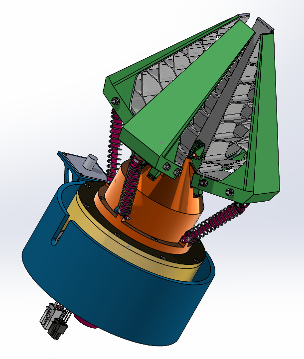
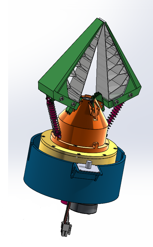
Figure 1a: Full assembly of four-jaw configuration blah Figure 1b: Full assembly of two-jaw configuration
A planetary gearbox ensures the rotation of the gripper around its centre axis. The sun gear allows for the cables of the jaws motor and force sensors to connect to the rest of the system. The wrist pitch is actuated by a DC motor combined with a planetary gear head. The gear head is connected to a 1:1 pulley-belt drive. Overall, the gripper utilises three DC motors, three encoders, three motor drivers, and two force sensors. Additionally, the gripper carries a camera used for Business Logic during maintenance and sampling tasks. The video feed is sent to the computer vision system.
All components and their CAD models are listed in the Excel sheet located in the drive:
Or by clicking on the following link:
https://docs.google.com/spreadsheets/d/1X3AsVIhJ1_YzZIhLjmNuEIaihkdtOWf1gauOEwgxZvM/edit?usp=sharing
4. Current Challenges (ERC 2026)
During the prototyping and integration phases, several issues were identified in the current gripper design:
- Housing fragility: The current housing of the worm gear has been the main breaking point of all prototypes. Specifically, the housing breaks at the connection point between the worm wheels and the housing, especially when the gripper faces resistance and must provide higher torque.
- Planetary gearbox connection: The planetary gearbox is very difficult to assemble and, hence, to troubleshoot in case of damage. This issue is also time-consuming and unpredictable, as components can break during assembly and require a newl printed components.
- Wrist connection: The connection of the gripper to the rest of the arm is done by a bracket that is attached to a belt drive system (wrist connection). The wrist connection is currently wiggly, which leads to inaccurate control. Additionally, the connection to the gripper is relatively complicated.
- Inefficient configuration change: To change from one configuration to another, the users must retrieve M2 bolts and nuts. By taking out the bolts and nuts, the spring assemblies are completely disconnected and very easy to lose. Additionally, the M2 bolts and nuts are challenging to reassemble.
- Sensor absence: Due to time constraints, the force sensors on the jaws' reinforcements were never integrated with the gripper.
- Water-tight camera container: The container was printed as a quick prototype, where hot glue was used to create watertightness. Because the glue was unevenly applied, the camera holder could leak and damage the camera.
5. Ideas & Future Improvements
- Automatic configuration change: To solve the inefficient configuration change, the housing could be modified to create an automatic configuration change mechanism. The challenge of this project is to implement an actuator that can roughly fit within the current design. Another challenge is the design of the housing to mechanically follow the actuation without breaking any permanent connection.
- Redesign of the housing: The housing must also be redesigned to guarantee that it will be able to support the high torque transmitted by the jaws on the manipulated object without breaking. During this redesign, the goal should also be to preserve the sturdy connection with the DC motor and planetary gearbox.
- Redesign of the connection point of the planetary gearbox: Connecting the planetary gearbox with its actuator and the bottom plate of the gripper remains quite inefficient for several reasons. First, Loctite is applied on the three M4 'shafts' (currently threaded rods within the prototype) to lock the nuts in place and ensure they do not fall out of the system due to the rotation of the gearbox. Then, the Loctite is a relatively permanent connection. Hence, in case a gear must be replaced, one must pour and rub acetone on the nuts and pull in very chaotic ways to disassemble the bottom plate and access the rest of the system. Improving the connection mechanism of the planetary gearbox with the rest of the system will make the gripper easier to analyse, fix and improve.
- Redesign of wirst connection to the belt drive: To fix the wrist connection, one must redesign the brackets, especially the connection to the gripper. Another solution would be to replace the brackets with one piece connected at the centre of the gripper and the centre of the actuated shaft in the belt drive system. Further research on potential solutions could be done by performing a literature review on robotic wrist design articles.
- Improvement of the watertightness of the camera holder: The camera cap should be connected with four screws instead of two. Additionally, a TPU insert could be added as a guarantee that no leakage will occur.
- Modular gripper: Similar to the automatic configuration change, making this design modular to be able to exchange the type of jaws or add a scoop for regolith manipulation, or even exchange the jaws with a tube holder to safely collect liquid with the liquid collector (see chassis book).